《复仇者联盟4》终于上映,这部汇集了10年回忆打造的电影,据看过的小伙伴们表示:3小时剧情,毫无尿点,全程都是经典回忆。
忙着工作还没来得及看电影,又超怕被剧透的文摘菌这两天的状态基本是这样
万般捉急的文摘菌在这周也去重新回忆了一下这个系列的作品。这部电影是复仇者系列的终结作品,能有如此成就,离不开《钢铁侠》、《美国队长》,《雷神》、《绿巨人》等独立叙事电影为其构建的宏大的宇宙观,也在全球观众心里种下同一种英雄情结。
复仇者系列火遍全球绝非意外,这部作品尽管出现了各种人物,但是每个英雄又都被塑造地各具特色,让人一次就能记住。
而台词可以说是最能塑造人物性格的部分了。因此,文摘菌希望用数据分析的方式,看看漫威宇宙的英雄最爱用的词汇可视化,并通过此分析他们的人物特点,向这部伟大的作品致敬。
本次分析,我们主要使用了R语言进行编程,目的是找出最能代表每位英雄的词汇。数据选用了三个比较有代表性的漫威英雄交叉度极高的剧本,分别是:《复仇者联盟》(就是打洛基的那一部)、《复仇者联盟:奥创纪元》以及《美国队长:内战》。
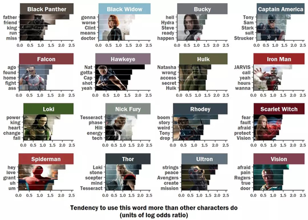
上代码前,先来看看分析结果。
1. 美国队长:以你的名字呼唤你-钢铁侠!

作为联盟的老大哥,美国队长超爱喊别人的名字。并且我们发现,他口中最经常出现的名字就是钢铁侠。此外,还经常点名的是Sam,和Strucker。

美国队长和钢铁侠可谓《复仇者联盟》系列中两大相爱相杀的主角了。两人在电影中都是领导级别的角色,但是两者的追求却有很大的差异。在电影《美国队长:内战》中,复仇者联盟团队彻底分崩离析,分别从属了美国队长和钢铁侠两大阵营。
一方面美国队长为了自己的好朋友冬兵战斗,另一方钢铁侠为了维护世界的秩序和为自己的父母报仇战斗。两者即是好友,又是同级别的对手,这或许也就解释了为什么美国队长总是叫钢铁侠的名字。
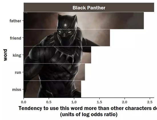
2. 黑豹:最喜欢谈论“中二“话题的贵族
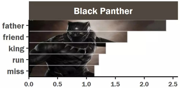
从分析结果来看,黑豹最喜欢说的是父亲、朋友,国王等听起来比较“中二“的词语。

黑豹的父亲前任黑豹特查卡,瓦坎达的国王!守护者振金,是黑豹的偶像,却在电影中死于一场阴谋。而黑豹作为瓦坎达的领袖,年轻的王位继承人,将他父亲的遗志作为了追求的梦想,守护着瓦坎达。国王身份,追求理想,这就是黑豹喜欢谈论这类贵族话题的原因。
3. 蜘蛛侠:我还是个“宝宝“。

作为全队的“小朋友“,蜘蛛侠在复仇者联盟系列电影中的台词一直比较幼齿,他在电影中说的最多的是词是:“嗨”、“呃”、“嗯”。
在这三部电影中,蜘蛛侠只是一个十几岁的孩子,在这么多大人物面前如果再不蹦蹦跳跳,那就更没有存在感了☺。
4. 浩克和鹰眼:大家都爱黑寡妇。
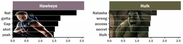
通过可视化分析可以发现,绿巨人和鹰眼都非常喜欢提到黑寡妇。

浩克喜欢和黑寡妇聊天原因很简单,因为当绿巨人发狂时,黑寡妇用满心关爱的眼神瞅着他那庞大的身躯,对他说道:“嘿,大块头,太阳快下山了!”然后慢慢地举起了手,用她那柔软的手指,伸向了绿巨人的手臂,轻轻滑了下来。这时候浩克就会平息他那满腔的怒火!
电影中黑寡妇和鹰眼不是恋人或者情侣,他们的关系一直恋人未满、暧昧不清。但是,因为两人在复仇者联盟之前就已经发生了一系列故事。刀光剑影,爱恨情仇,即是老友又是战友,或许两人早已暗生情愫。
5. 幻世和绯红女巫:惺惺相惜,在线发糖!

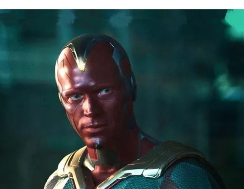
从数据可视化的结果中可以看到,幻视和绯红女巫绝对是soulmate了,两人的谈论内容都很一致,特别喜欢说“恐惧、担忧“类话题!
关于绯红女巫,我们可以从她童年的经历和非人的待遇中找到原因。而幻世作为超级人工智能,能够看到别的英雄看不到的“画面”,可能对未来的担忧让他心烦意乱。
6. 托尔:能力越大,责任越大,考虑深远

托尔作为雷神,拥有多种魔法能力,例如:操控风暴,释放或控制闪电,将闪电能量实体化为盔甲,瞬间改变天气,利用雷神之锤飞行,召唤雷神之锤令其飞回托尔用闪电与敌人交战。

雷神除去强大的战斗力,托尔还掌握着星际级的知识。例如:无限宝石知识、各式星际飞船驾驶技术、格鲁特语(格鲁特所在种族的语言)、虫洞知识。
或许是能力越大,责任越大,他比其他英雄角色看的更远。在电影中,他对推动剧情前进的物品更加专注,例如洛基的权杖以及心灵宝石。
7. 洛基:追逐权力。

洛基从小和雷神托尔一起长大。一直窥视众神之王的宝座且不认同雷神托尔会是一位合格的继承人。他野心十足想当老大,阴险狡诈陷害兄长、反逆父母,视天下生命如草芥,为了目的不择手段。
总之一句话,他非常想要权力!
8. 奥创:更爱“诗和远方“。

奥创被制造出来的目的是为了守护和平,但是一诞生就发生错误,认为想要和平就要消灭人类和复仇者联盟,于是抢走洛基权杖(心灵宝石)从尤利西斯·克劳手中弄到大量的振金,操纵赵海伦利用再生摇篮帮其制造幻视身体,想要进化得更强。
换句话说,奥创一出生就被订上了守护和平的烙印,虽然他看问题的角度不同,但是和复仇者联盟有着共同的任务。所以,它更加向往诗与远方!

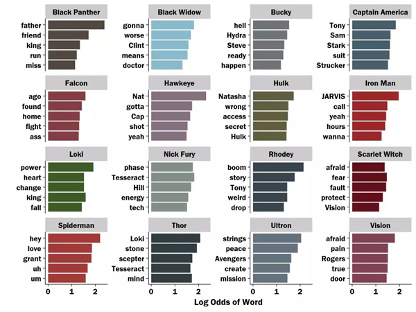
上面条条的长度对应的是超级英雄使用每个词汇的程度。
可视化过程
最后,分析完全剧的角色,我们也来一起看看整个可视化过程。
导入R语言包:
library(dplyr) library(grid) library(gridExtra) library(ggplot2) library(reshape2) library(cowplot) library(jpeg) library(extrafont)
清除R工作环境中的全部东西:
rm(list = ls())
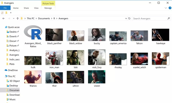
加载包含所有图片的文件夹(根据你自己的情况修改代码):
dir_images <- "C:\\Users\\Matt\\Documents\\R\\Avengers" setwd(dir_images)
设置字体:
windowsFonts(Franklin=windowsFont("Franklin Gothic Demi"))
英雄角色名字的简化版本:
character_names <- c("black_panther","black_widow","bucky","captain_america", "falcon","hawkeye","hulk","iron_man", "loki","nick_fury","rhodey","scarlet_witch", "spiderman","thor","ultron","vision") image_filenames <- paste0(character_names, ".jpg")
将所有图片读入一个列表中。
all_images <- lapply(image_filenames, read_image)
将角色名字分配给图像列表,以便按名字对其进行索引。
names(all_images) <- character_names
例如:
# clear the plot window grid.newpage() # draw to the plot window grid.draw(rasterGrob(all_images[['vision']]))
获得文本数据
数据由计算机科学家Elle O'Brien收集的,使用文本挖掘技术对电影剧本分析。
更正专有名称的大写:
capitalize <- Vectorize(function(string){ substr(string,1,1) <- toupper(substr(string,1,1)) return(string) }) proper_noun_list <- c("clint","hydra","steve","tony", "sam","stark","strucker","nat","natasha", "hulk","tesseract", "vision", "loki","avengers","rogers", "cap", "hill") # Run the capitalization function word_data <- word_data %>% mutate(word = ifelse(word %in% proper_noun_list, capitalize(word), word)) %>% mutate(word = ifelse(word == "jarvis", "JARVIS", word))
请注意,以前的简版角色名字与文本dataframe格式中的角色不匹配。
unique(word_data$Speaker) ## [1] "Black Panther" "Black Widow" "Bucky" ## [4] "Captain America" "Falcon" "Hawkeye" ## [7] "Hulk" "Iron Man" "Loki" ## [10] "Nick Fury" "Rhodey" "Scarlet Witch" ## [13] "Spiderman" "Thor" "Ultron" ## [16] "Vision"
创建一个索引表,将文件名转换为角色名。
character_labeler <- c(`black_panther` = "Black Panther", `black_widow` = "Black Widow", `bucky` = "Bucky", `captain_america` = "Captain America", `falcon` = "Falcon", `hawkeye` = "Hawkeye", `hulk` = "Hulk", `iron_man` = "Iron Man", `loki` = "Loki", `nick_fury` = "Nick Fury", `rhodey` = "Rhodey",`scarlet_witch` ="Scarlet Witch", `spiderman`="Spiderman", `thor`="Thor", `ultron` ="Ultron", `vision` ="Vision")
有两个不同版本的角色名,一个用于显示(漂亮),一个用于索引(简单)。
convert_pretty_to_simple <- Vectorize(function(pretty_name){ # pretty_name = "Vision" simple_name <- names(character_labeler)[character_labeler==pretty_name] # simple_name <- as.vector(simple_name) return(simple_name) }) # convert_pretty_to_simple(c("Vision","Thor")) # just for fun, the inverse of that function convert_simple_to_pretty <- function(simple_name){ # simple_name = "vision" pretty_name <- character_labeler[simple_name] %>% as.vector() return(pretty_name) } # example convert_simple_to_pretty(c("vision","black_panther"))
## [1] "Vision" "Black Panther"
将简化的角色名称添加到文本数据框架中。
word_data$character <- convert_pretty_to_simple(word_data$Speaker)
为每个角色指定主颜色:
character_palette <- c(`black_panther` = "#51473E", `black_widow` = "#89B9CD", `bucky` = "#6F7279", `captain_america` = "#475D6A", `falcon` = "#863C43", `hawkeye` = "#84707F", `hulk` = "#5F5F3F", `iron_man` = "#9C2728", `loki` = "#3D5C25", `nick_fury` = "#838E86", `rhodey` = "#38454E",`scarlet_witch` ="#620E1B", `spiderman`="#A23A37", `thor`="#323D41", `ultron` ="#64727D", `vision` ="#81414F" )
绘制条形图
avengers_bar_plot <- word_data %>% group_by(Speaker) %>% top_n(5, amount) %>% ungroup() %>% mutate(word = reorder(word, amount)) %>% ggplot(aes(x = word, y = amount, fill = character))+ geom_bar(stat = "identity", show.legend = FALSE)+ scale_fill_manual(values = character_palette)+ scale_y_continuous(name ="Log Odds of Word", breaks = c(0,1,2)) + theme(text = element_text(family = "Franklin"), # axis.title.x = element_text(size = rel(1.5)), panel.grid = element_line(colour = NULL), panel.grid.major.y = element_blank(), panel.grid.minor = element_blank(), panel.background = element_rect(fill = "white", colour = "white"))+ # theme(strip.text.x = element_text(size = rel(1.5)))+ xlab("")+ coord_flip()+ facet_wrap(~Speaker, scales = "free_y") avengers_bar_plot
这已经非常漂亮了,但是还可以更漂亮。比如人物形象通过“线条”显示出来。具体做法是将透明的条形图全覆盖,然后从端点向里绘制白色的条形图,注意条形图是能够遮挡图片的。
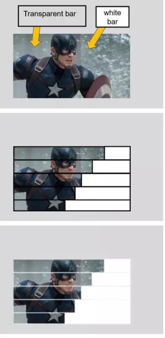
在数据框架中,用达到总最大值所需的余数来补充数值,这样当将值和余数组合在一起时,就会形成长度一致的线条组合。
max_amount <- max(word_data$amount) word_data$remainder <- (max_amount - word_data$amount) + 0.2
每个英雄角色仅提取5个关键词。
word_data_top5 <- word_data %>% group_by(character) %>% arrange(desc(amount)) %>% slice(1:5) %>% ungroup()
将“amount”和“remaining”的格式进行转换:
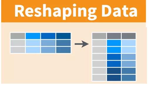
确保每个角色有两个长条;一个用于显示amount,另一个用于选择结束位置。
这会将“amount”和“remaining”折叠成一个名为“variable”的列,指示它是哪个值,另一列“value”包含每个值中的数字。
word_data_top5_m <- melt(word_data_top5, measure.vars = c("amount","remainder"))
将这些条形图放在有序因素中,与在数据融合中相反。否则,“amount”和“remainder”将在图上以相反的顺序显示。
word_data_top5_m$variable2 <- factor(word_data_top5_m$variable, levels = rev(levels(word_data_top5_m$variable)))
每个角色仅仅显示五个词汇
注意角色名称的版本问题,例如采用“black_panther”而不是“Black Panther”。
plot_char <- function(character_name){ # example: character_name = "black_panther" # plot details that we might want to fiddle with # thickness of lines between bars
bar_outline_size <- 0.5 # transparency of lines between bars bar_outline_alpha <- 0.25 # # The function takes the simple character name, # but here, we convert it to the pretty name, # because we'll want to use that on the plot. pretty_character_name <- convert_simple_to_pretty(character_name) # Get the image for this character, # from the list of all images. temp_image <- all_images[character_name] # Make a data frame for only this character temp_data <- word_data_top5_m %>% dplyr::filter(character == character_name) %>% mutate(character = character_name) # order the words by frequency # First, make an ordered vector of the most common words # for this character ordered_words <- temp_data %>% mutate(word = as.character(word)) %>% dplyr::filter(variable == "amount") %>% arrange(value) %>% `[[`(., "word") # order the words in a factor, # so that they plot in this order, # rather than alphabetical order temp_data$word = factor(temp_data$word, levels = ordered_words) # Get the max value, # so that the image scales out to the end of the longest bar max_value <- max(temp_data$value) fill_colors <- c(`remainder` = "white", `value` = "white") # Make a grid object out of the character's image character_image <- rasterGrob(all_images[[character_name]], width = unit(1,"npc"), height = unit(1,"npc")) # make the plot for this character output_plot <- ggplot(temp_data)+ aes(x = word, y = value, fill = variable2)+ # add image # draw it completely bottom to top (x), # and completely from left to the the maximum log-odds value (y) # note that x and y are flipped here, # in prep for the coord_flip() annotation_custom(character_image, xmin = -Inf, xmax = Inf, ymin = 0, ymax = max_value) + geom_bar(stat = "identity", color = alpha("white", bar_outline_alpha), size = bar_outline_size, width = 1)+ scale_fill_manual(values = fill_colors)+ theme_classic()+ coord_flip(expand = FALSE)+ # use a facet strip, # to serve as a title, but with color facet_grid(. ~ character, labellerlabeller = labeller(character = character_labeler))+ # figure out color swatch for the facet strip fill # using character name to index the color palette # color= NA means there's no outline color. theme(strip.background = element_rect(fill = character_palette[character_name], color = NA))+ # other theme elements theme(strip.text.x = element_text(size = rel(1.15), color = "white"), text = element_text(family = "Franklin"), legend.position = "none", panel.grid = element_blank(), axis.text.x = element_text(size = rel(0.8)))+ # omit the axis title for the individual plot, # because we'll have one for the entire ensemble theme(axis.title = element_blank()) return(output_plot) }
单个角色是如何设置?
sample_plot <- plot_char("black_panther")+ theme(axis.title = element_text())+ # x lab is still declared as y lab # because of coord_flip() ylab(plot_x_axis_text) sample_plot
横轴为什么这么特殊?因为随着数值的增加,条形图会变得越来越高,因此需要转换刻度。
如下所示
logit2prob <- function(logit){ odds <- exp(logit) prob <- odds / (1 + odds) return(prob) }
…这就是这个轴的样子:
logit2prob(seq(0, 2.5, 0.5))
## [1] 0.5000000 0.6224593 0.7310586 0.8175745 0.8807971 0.9241418
注意该列表中连续项之间的递减差异:
diff(logit2prob(seq(0, 2.5, 0.5)))
## [1] 0.12245933 0.10859925 0.08651590 0.06322260 0.04334474
好了,可以进行下一项了:探讨一些细节,并把上面设置的函数应用到所有角色的列表中,并把所有的结果放入一个列表中。
all_plots <- lapply(character_names, plot_char)
从图片中提取标题
get_axis_grob <- function(plot_to_pick, which_axis){ # plot_to_pick <- sample_plot tmp <- ggplot_gtable(ggplot_build(plot_to_pick)) # tmp$grobs # find the grob that looks like # it would be the x axis axis_x_index <- which(sapply(tmp$grobs, function(x){ # for all the grobs, # return the index of the one # where you can find the text # "axis.title.x" or "axis.title.y" # based on input argument `which_axis` grepl(paste0("axis.title.",which_axis), x)} )) axis_grob <- tmp$grobs[[axis_x_index]] return(axis_grob) }
提取轴标题:
px_axis_x <- get_axis_grob(sample_plot, "x") px_axis_y <- get_axis_grob(sample_plot, "y")
下面是如何使用提取出来的坐标轴:
grid.newpage() grid.draw(px_axis_x)
# grid.draw(px_axis_y)
汇总所有的英雄:
big_plot <- arrangeGrob(grobs = all_plots)
加入图注,注意图和坐标轴的比例关系:
big_plot_w_x_axis_title <- arrangeGrob(big_plot, px_axis_x, heights = c(10,1)) grid.newpage() grid.draw(big_plot_w_x_axis_title)

因为词汇的长度不同,这些图表占用的页面空间略有不同。
所以,这看起来有点乱。
一般来说,我们使用facet_grid()或facet_wrap()确保在绘图的过程中保持整齐和对齐,这个项目中不再适用,因为每个都有自己的自定义背景图像。
使用Cowplot而不是arrangebrob,让图片的轴垂直对齐:
big_plot_aligned <- cowplot::plot_grid(plotlist = all_plots, align = 'v', nrow = 4)
增加X轴的标题,和之前类似,注意网格对齐:
big_plot_w_x_axis_title_aligned <- arrangeGrob(big_plot_aligned, px_axis_x, heights = c(10,1))
然后,大功告成
然后,保存一下!
ggsave(big_plot_w_x_axis_title_aligned, file = "Avengers_Word_Usage.png", width = 12, height = 6.3)
(文章来源:大数据文摘)

